DATA 310: Applied Machine Learning
Course ID: DATA 310
Course Attribute: None
Title: Applied Machine Learning
Credit Hours: 3
Meeting Times: 10:10 to 12:00 MTWTh
Location: Remote Synchronous Off-Campus
Date Range: Summer II Semester 2021
Course Description
This course will focus on the technical application of machine learning algorithms, their nature, and discussions regarding the potential drawbacks and advantages of different classes of algorithms. Students entering into this course should have, at a minimum, a background in python and linear algebra. No single algorithm will be covered in great depth, and the course will place a focus on the code and implementation choices necessary for each class of algorithm. Topics covered will include data processing, regression in ML, decision trees, forests, k-nn, support vector machines, kernel SVM, k-means and hierarchical clustering, association rules, natural language processing, neural networks, and various associated approaches. Pre-requisite(s): (DATA 141 OR DATA 140 OR CSCI 140 OR CSCI 141) AND (DATA 146 OR CSCI 146)
Goals and Objectives:
- To provide students with a critical understanding of the variety of tools that can be used for machine learning.
- To develop students ability to communicate findings, analysis, and visualization skills for future courses (and jobs).
- To expose students to real-world problems that are being engaged with by contemporary problem solvers and decision makers.
Honor Code
Among our most significant traditions is the student-administered honor system. The Honor Code is an enduring tradition with a documented history that originates as far back as 1736. The essence of our honor system is individual responsibility. Today, students, such as yourself, administer the Honor pledge to each incoming student while also serving to educate faculty and administration on the relevance of the Code and its application to students’ lives.
The Pledge
“As a member of the William and Mary community, I pledge on my honor not to lie, cheat, or steal, either in my academic or personal life. I understand that such acts violate the Honor Code and undermine the community of trust, of which we are all stewards.”
Accessibility, Attendance & Universal Learning
William & Mary accommodates students with disabilities in accordance with federal laws and university policy. Any student who feels s/he may need accommodation based on the impact of a learning, psychiatric, physical, or chronic health diagnosis should contact Student Accessibility Services staff at 757-221-2509 or at sas@wm.edu to determine if accommodations are warranted and to obtain an official letter of accommodation. For more information, please see www.wm.edu/sas.
I am committed to the principle of universal learning. This means that our classroom, our virtual spaces, our practices, and our interactions be as inclusive as possible. Mutual respect, civility, and the ability to listen and observe others carefully are crucial to universal learning. Active, thoughtful, and respectful participation in all aspects of the course will make our time together as productive and engaging as possible.
Grade Categories
| exceptional A = 100 ≥ 97.0 | excellent A = 96.9 ≥ 93.0 | superior A- = 92.9 ≥ 90.0 |
| very good B+ = 89.9 ≥ 87.0 | good B = 86.9 ≥ 83.0 | above average B- = 82.9 ≥ 80.0 |
| normal C+ = 79.9 ≥ 77.0 | average C = 76.9 ≥ 73.0 | sub par C- = 72.9 ≥ 70.0 |
| below average D+ = 69.9 ≥ 67.0 | poor D = 66.9 ≥ 63.0 | very poor D- = 62.9 ≥ 60.0 |
| failing F < 60.0 |
note .9 = .9 with bar notation
Grading Opportunities
| Exercises | 40% | 4 modules |
| Projects | 40% | 4 projects |
| Final Project | 20% | due by 5PM on the last day of finals |
Semester Schedule
Week 1 (July 5)
-
Tuesday:
- 10:10 to 11:00 - Getting Started
- 11:00 to 11:30 - Small groups
- 11:30 to 12:00 - Reconvene
-
Wednesday:
- 10:10 to 11:00 - Exercise
- 11:00 to 11:30 - Small groups
- 11:30 - Close early
-
Thursday:
- 10:10 to 11:00 - Exercise
- 11:00 to 11:30 - Small groups
- 11:30 to 12:00 - Reconvene
-
Saturday:
- Informal Responses due by 5PM
-
Sunday:
- Project 1 due by 5PM
Week 2 (July 12)
-
Monday:
- 10:10 to 11:00 - Exercise
- 11:00 to 11:30 - Small groups
- 11:30 to 12:00 - Reconvene
-
Tuesday:
- 10:10 to 11:00 - Exercise
- 11:00 to 11:30 - Small groups
- 11:30 to 12:00 - Reconvene
-
Wednesday:
- 10:10 to 11:00 - Exercise
- 11:00 to 11:30 - Small groups
- 11:30 to 12:00 - Reconvene
-
Thursday:
- 10:10 to 11:00 - Exercise
- 11:00 to 11:30 - Small groups
- 11:30 to 12:00 - Reconvene
-
Saturday:
- Informal Responses due by 5PM
-
Sunday:
- Project 2 due by 5PM
Week 3 (July 19)
-
Monday:
- 10:10 to 11:00 - Exercise
- 11:00 to 11:30 - Small groups
- 11:30 to 12:00 - Reconvene
-
Tuesday:
- 10:10 to 11:00 - Exercise
- 11:00 to 11:30 - Small groups
- 11:30 to 12:00 - Reconvene
-
Wednesday:
- 10:10 to 11:00 - Exercise
- 11:00 to 11:30 - Small groups
- 11:30 to 12:00 - Reconvene
-
Thursday:
- 10:10 to 11:00 - Exercise
- 11:00 to 11:30 - Small groups
- 11:30 to 12:00 - Reconvene
-
Saturday:
- Informal Responses due by 5PM
-
Sunday:
- Project 3 due by 5PM
Week 4 (July 26)
-
Monday:
- 10:10 to 11:00 - Exercise
- 11:00 to 11:30 - Small groups
- 11:30 to 12:00 - Reconvene
-
Tuesday:
- 10:10 to 11:00 - Exercise
- 11:00 to 11:30 - Small groups
- 11:30 to 12:00 - Reconvene
-
Wednesday:
- 10:10 to 11:00 - Exercise
- 11:00 to 11:30 - Small groups
- 11:30 to 12:00 - Reconvene
-
Thursday:
- 10:10 to 11:00 - Exercise
- 11:00 to 11:30 - Small groups
- 11:30 to 12:00 - Reconvene
-
Saturday:
- Informal Responses due by 5PM
-
Sunday:
- Project 4 due by 5PM
Week 5 (August 2)
-
Monday:
- 10:10 to 11:00 - Exercise
- 11:00 to 11:30 - Small groups
- 11:30 to 12:00 - Reconvene
-
Tuesday:
- 10:10 to 11:00 - Exercise
- 11:00 to 11:30 - Small groups
- 11:30 to 12:00 - Reconvene
-
Wednesday:
- 10:10 to 11:00 - Exercise
- 11:00 to 11:30 - Small groups
- 11:30 to 12:00 - Reconvene
-
Thursday:
- 10:10 to 11:00 - Exercise
- 11:00 to 11:30 - Small groups
- 11:30 to 12:00 - Reconvene
-
Saturday:
- Informal Responses due by 5PM
-
Sunday:
- Final Project due by 5PM
Module 1
Tuesday
- Download and install python 3.9.6
The simplest way to install the latest version of python is by going to their website, python.org and downloading the most recent version. After arriving at the main python.org landing page you should find a tab linking to the download for Python 3.9.6. Once there, download and install the latest version of python for your Mac or Windows system. - Download and install PyCharm Professional Version
In this class we will use the integrated developer's environment (IDE), which goes by the name of PyCharm. Go to the jetbrains.org website and download the Professional version for your Mac or Windows system. After installing PyCharm, launch it from your applications folder. You can use the evaluate for free button for now, until you obtain your JetBrains educational license. - Set the python interpreter
After launching PyCharm, select new project, and give your project a name (perhaps DATA310), and for the python interpreter, select previously configured interpreter and choose the...tab to the right of the interpreter drop down menu. This tab will bring you to a new window, where you will want to select the system interpreter option on the left option bar. Hopefully the option for python3.9 already appears in the interpreter drop down menu. If not, you will likely need to select the...tab to the right again, and manually select the python3.9 interpreter from within your file system. On a Mac the path to the version of python you installed in step 1 is likely/usr/local/bin/python3.9. Once your python 3.9.6 interpreter has been selected, then click on the OK button in the bottom right hand corner.
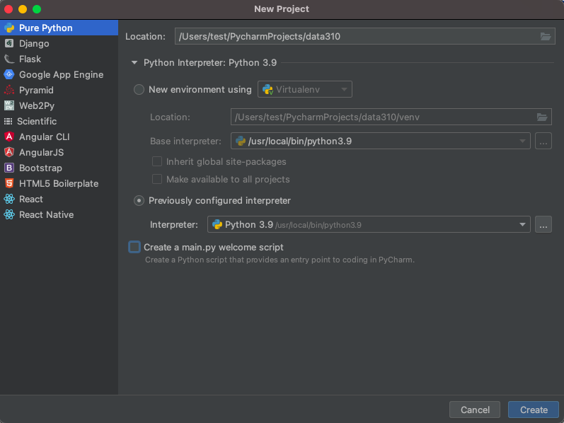
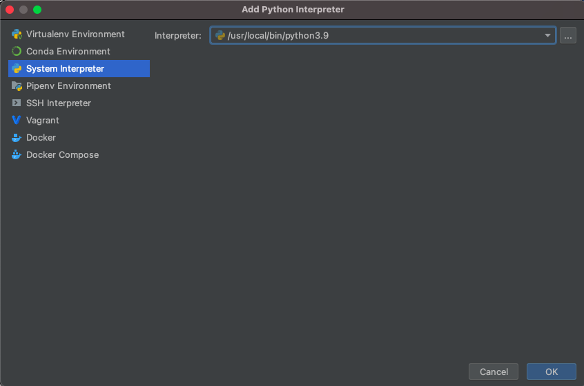
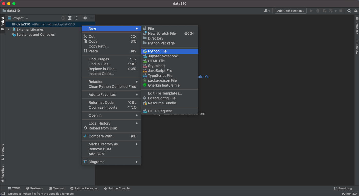
- Confirm your python session After creating a new script, click on the python console at the bottom of the screen and confirm your environment is using python 3.9.6. In your new script, add a line where you send a command to the interpreter.
2 + 2
The easiest way to execute the line of code is to make sure the cursor os on that line and then use the alt-shift-E combination in order to send the command to the interpreter for a result. Alternatively, you can option click (right click or two finger click) on the line and select the execute line in python console option.
If python returns the correct answer, then it appears you have properly configured your environment.
- Install a new package
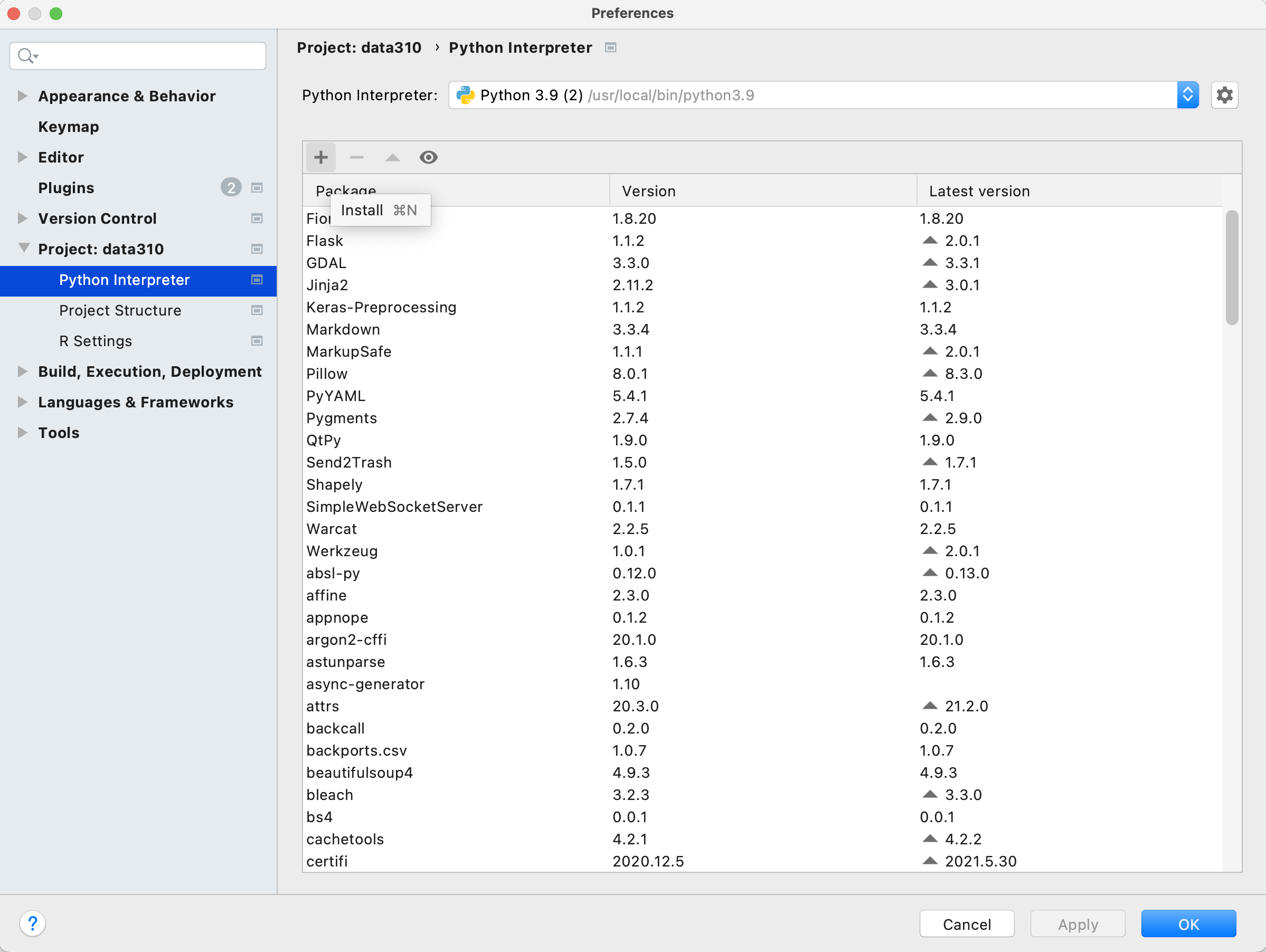
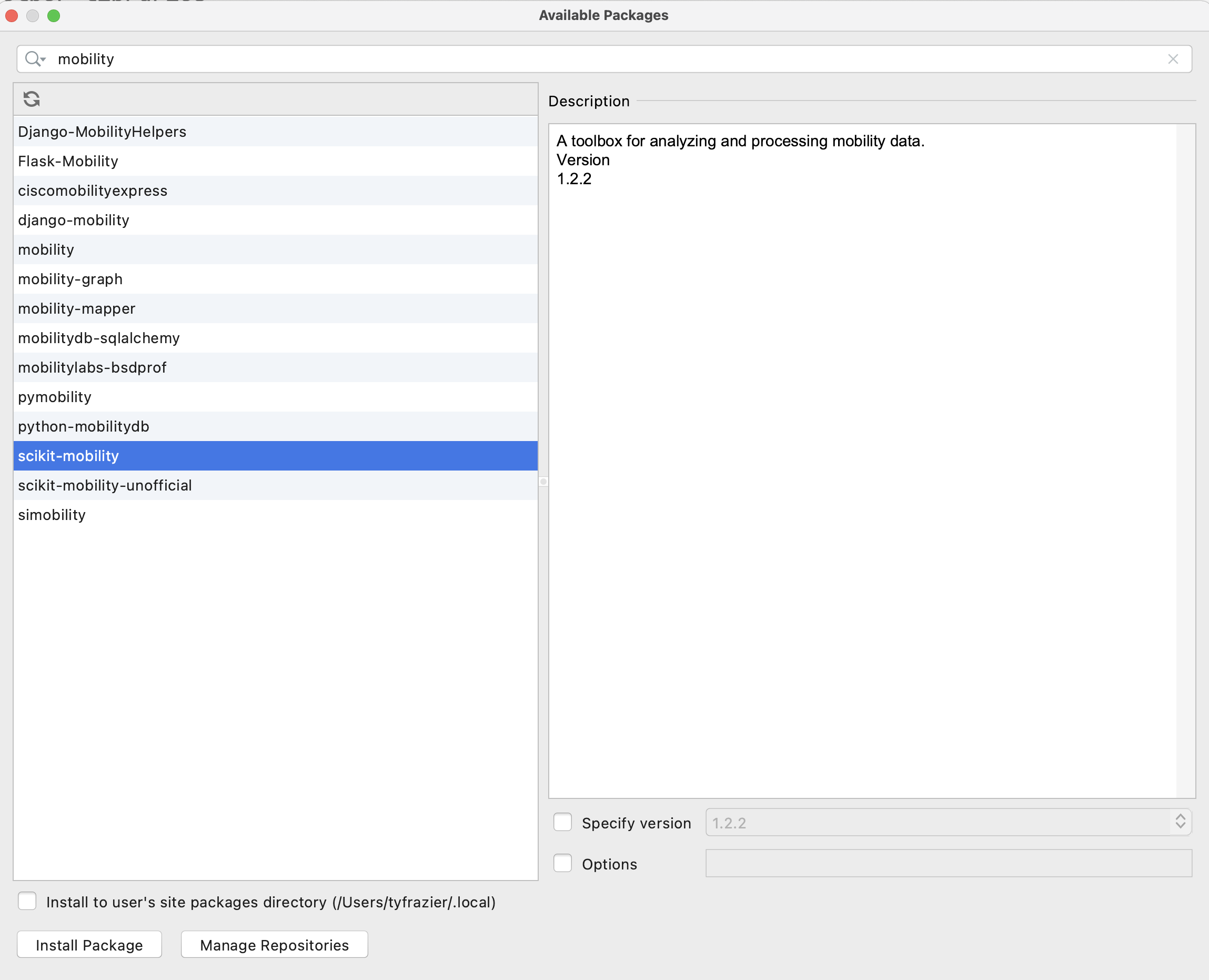
Your PyCharm IDE includes a package manager that makes package installation and updating fairly simple. To install a new package click on the preferences tab under your PyCharm pull down menu and then select the Project tab. Under the project tab you should see a subtab called Python Interpreter and off to the right, two packages that have already been installed. First, make sure both of these packages (should be pip and setuptools) have the most up to date version installed, and if not, use the up arrow symbol to upgrade each package to its latest version. Next select the + button to install a new package. Type tensorflow in the search window and then select install package. It might take a minute or two for the tensorflow package to complete its installation process. You can monitor your IDE's progress at the bottom while waiting for tensorflow to be installed successfully. After returning to main window of your package manager, you should notice a number of additional dependent packages that were installed in support of tensorflow. Close the system preferences window and add a new line to your script
import tensorflow. Again, your IDE may take a minute or two in order to execute the command for the first time, but once complete, you should see the>>>indication that your interpreter is ready to execute a command. If you click on the progress bar, it is possible to review the background tasks that involve updating the interpreter.
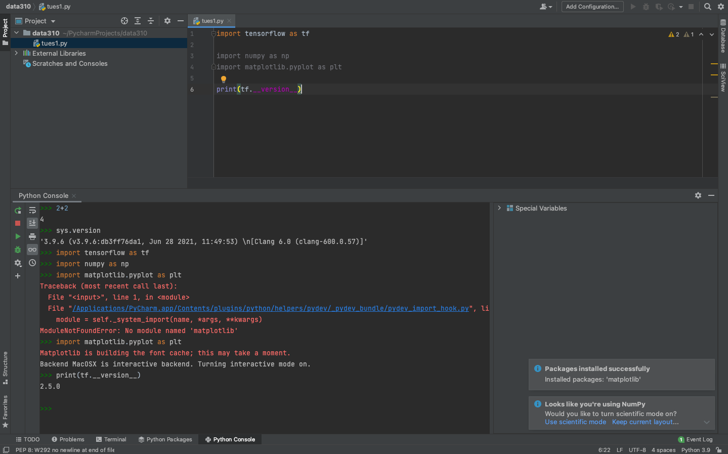
After the system finishes add a few lines to your script and confirm the output.
# TensorFlow and tf.keras
import tensorflow as tf

# Helper libraries
import numpy as np
import matplotlib.pyplot as plt

print(tf.__version__)
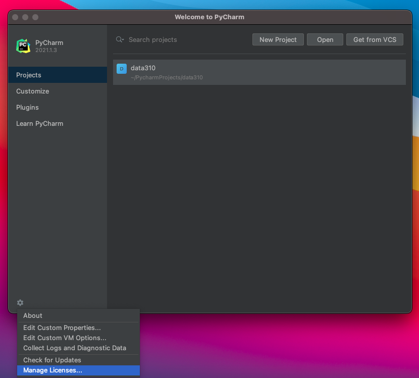
- Next go to the JetBrains webpage and register for an educational license. After receiving your license, return to the Welcome to PyCharm page and click on the gear symbol in the bottom left hand corner, where you will find the option to manage licenses. Enter your license to register your Professional version of PyCharm.
-
Next install the JetBrains IDE WebStorm for interacting with your GitHub account. Webstorm is a good IDE for producing markdown files for publishing in your public facing GitHub pages site.
-
Next, if you don't already have one, create a GitHub account. Once you have a GitHub account, create a new repository. Perhaps call it data310. Each repository needs to have a
README.mdfile in its root directory. Be sure to create one, which you can use as the index for your repository of formal and informal assignments. -
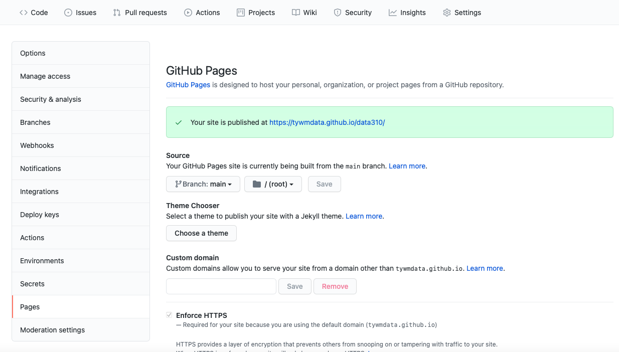
Go to the settings tab in your repository and click on the pages tab in the left hand pane. Set the branch to main, save your GitHub pages and then note where your site has been published. Click on the link and reload it, until it appears. Sometimes this can take a minute or two.
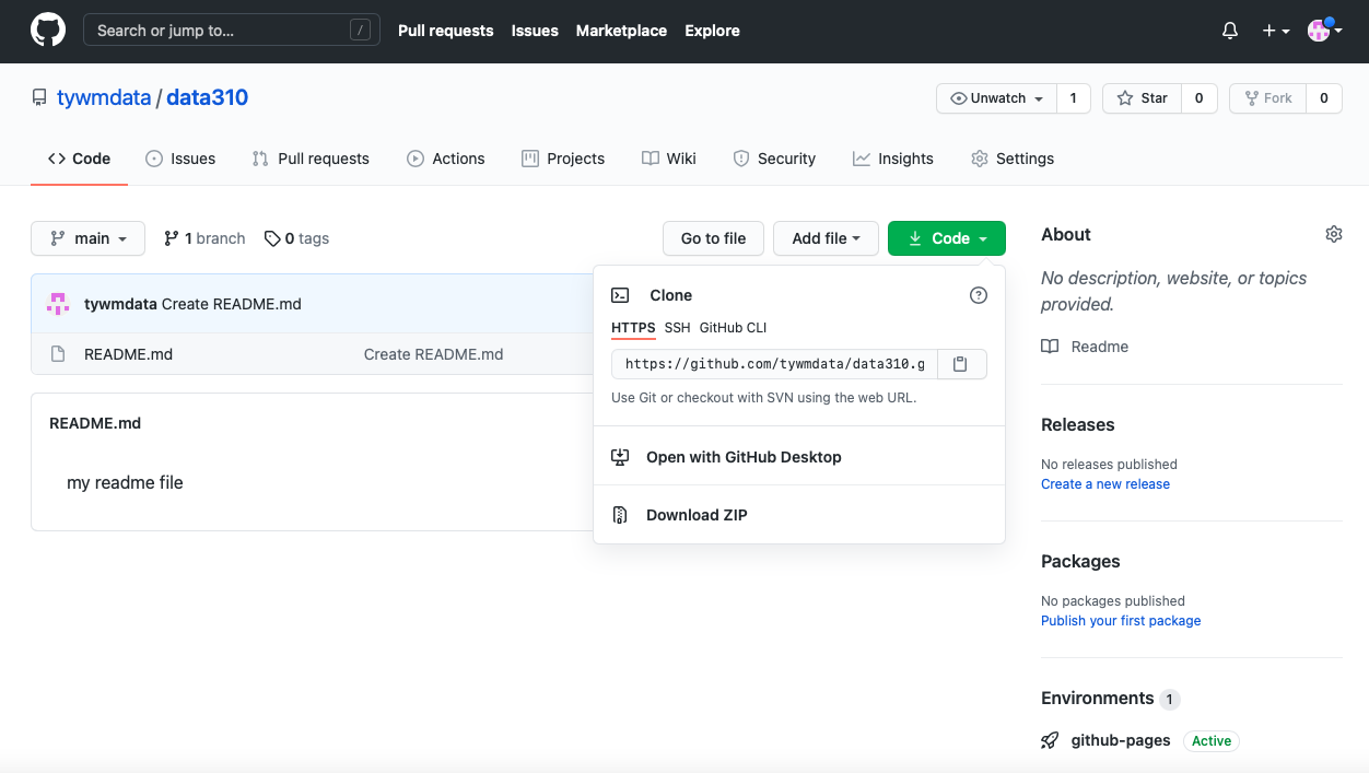
- In the main page of your repository open the code tab and copy the HTTPS address that you will use to link your repository to WebStorm via version control. Go back to the Welcome to Webstorm page and select the Get from VCS tab. Paste your HTTPS address into the URL field in order to clone your GitHub pages repository.
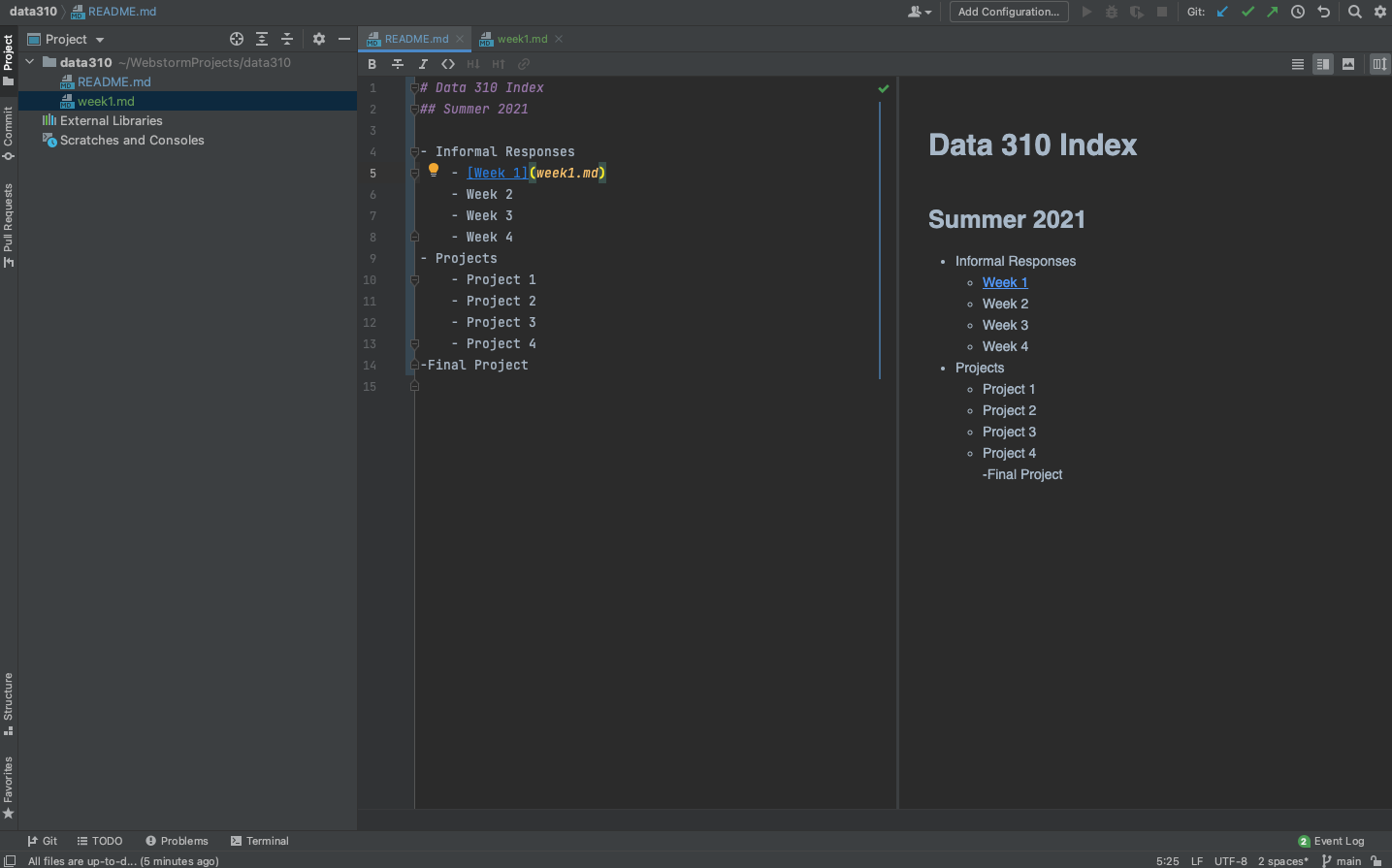
- Once you have cloned the repository from your GitHub account, you have a local project that can be modified and then those changes can be pushed to the GitHub repo for publishing via GitHub Pages (which happens automatically through something called the Jekyll engine). Go ahead and modify your
README.mdfile by setting it up as the index for your informal and formal assignments. Perhaps your index looks something like the following. Note how I created thewwek1.mdfile and linked it in the index.
Markdown is fairly simple to learn. Here is a guide.
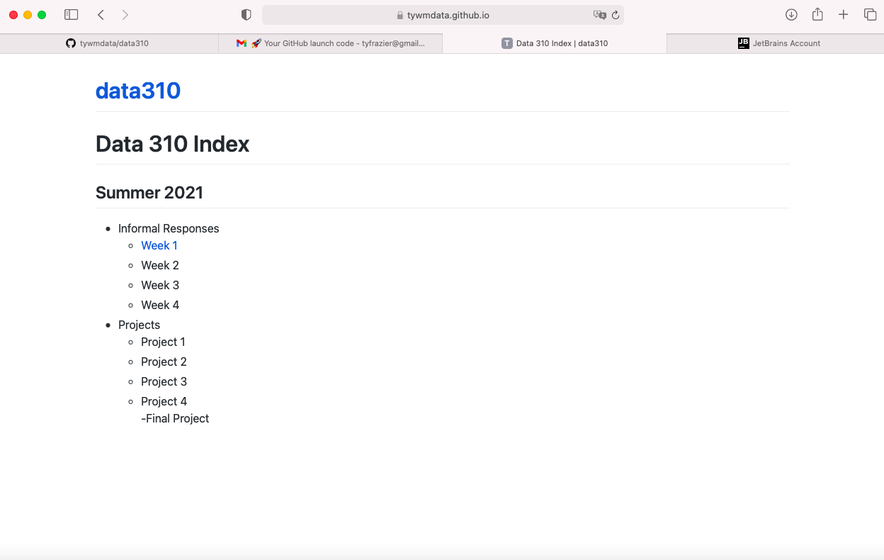
Now push those changes to your repository by selecting the commit tab on the left hand side, highlighting all the falls you have changed to commit, add a commit message , and then select the commit and push tab. You may need to add your user name, e-mail and authorize your account. Now go back to your GitHub pages webaddress and notice that the changes have taken place.
- Finally, go back to PyCharm and create a new python script. Go to the tensorflow webpage at https://www.tensorflow.org/tutorials/keras/classification, read and reproduce the script in PyCharm and run it. Answer the following questions about the dataset.
- What is the shape of the images training set (how many and the dimension of each)?
- What is the length of the labels training set?
- What is the shape of the images test set?
Be prepared to discuss during tomorrow's class.
Wednesday
Start with the Basic classification: Classify images of clothing script that you prepared for today's class. Execute the following.
- From the Preprocess the data section of the script, modify the training image to produce three new images.
- Under the Make predictions section, present the array of predictions for an image from the test set other than the one given in the example script. What does this array represent? How were the
Softmax()andargmax()functions applied? Read this post from DeepAI, What is the Softmax function for a description of the two functions (focus on the softmax formula, calculating softmax and the softmax vs. argmax sections). Does the output fromnp.argmax()match the label from yourtest_labelsdataset? - Under the Verify predictions section, plot two additional images (other than either of the two given in the example script) and include the graph of their predicted label as well as the image itself.
- Under the Use the trained model section, again select a new image from the test dataset. Produce the predictions for this newly selected image. Does the predicted value match the test label? Although you applied the
argmax()function in this second instance, you did not useSoftmax()a second time. Why is that so (please be specific)?
Copy the script you produced for the Fashion MNIST dataset. Modify the script as follows and produce the following output.
- Change the line
fashion_mnist = tf.keras.datasets.fashion_mnist
to
mnist = tf.keras.datasets.mnist
in order to switch the dataset from sets of clothing to hand written numbers. Produce a plot of 25 handwritten numbers from the data with their labels indicated below each image. Fit the model and report the accuracy of the training dataset. Likewise report the accuracy of the test dataset. As in the above example, from the Verify predictions section, plot two images and include the graph of their predicted label as well as the image itself.
- Evaluate how your model for the MNIST dataset compared with your model of the Fashion_MNIST dataset. Which of the two models is more accurate? Why do you think this is so?
For Thursday's class, reproduce the script on Basic Text Classification. Please read through the script and confirm you are able to execute a basic inferential sentiment analysis.
Thursday
At the bottom of the Basic Text Classification exercise you prepared for today's class is a second similarly structured exercise. With two of your classmates, complete the multi-class classification on Stack Overflow questions exercise.
- Provide plots that describe the training and validation loss and accuracy. Interpret the plots. How is this model performing?
- Export the model and print the accuracy produced using the test data. Does the test data accuracy serve to validate your model?
- Produce three examples that are relevant to the multi-class classification model and predicting the language relevant to the stack overflow question. Produce the array generated by each of your three examples. Were these predictions accurate?
- Compare your multi-class model with your binary class model that predicted sentiment as either positive or negative in response to various movie reviews. What is the most significant difference between the two different types of models? Compare the two models and estimate which demonstrated better performance? Substantiate your response.
Project 1
Collect data from zillow to train a model that predicts home price.
- For reference watch What is ML by Laurence Maroney, beginning at about minute 8 with the subsequent housing price exercise presented at the end of the video. You are also welcome to refer to the beginning part of the second video in this series First steps in computer vision, where the solution to the example housing price exercise is presented.
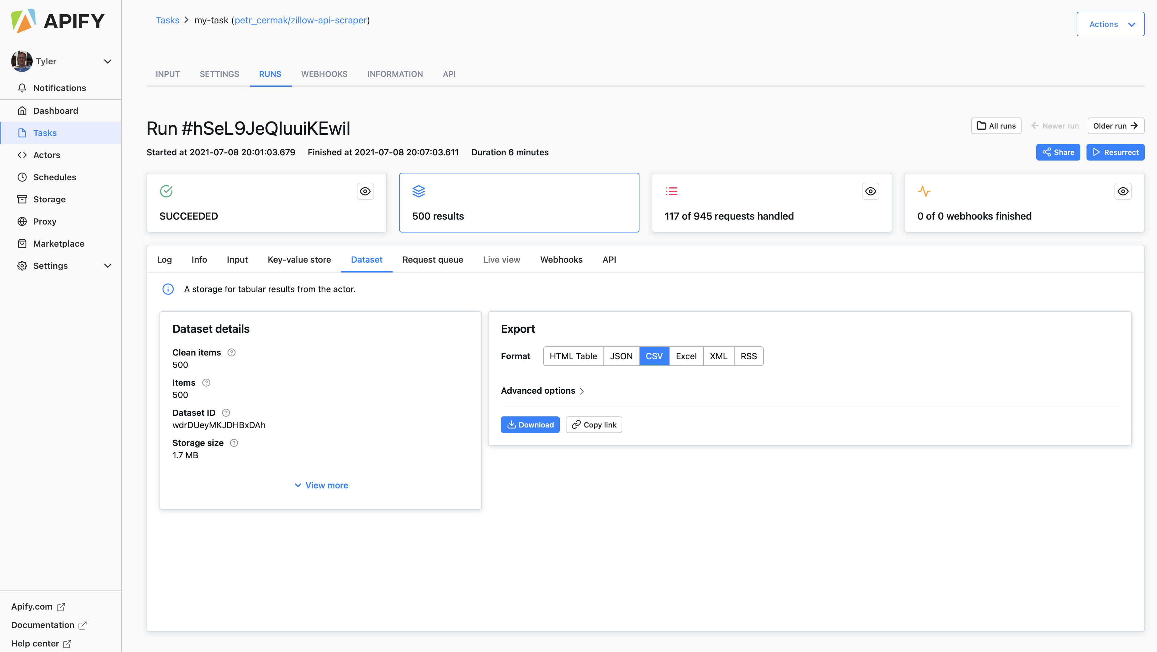
- Got to the Apify zillow scraper and scrape a few hundred home sale listings from any city. Download the file as a
.csv.
-
Use the pandas
read_csv()function to import your file to your PyCharm session. Create a data frame that has the following variables.- price
- bedrooms
- bathrooms
- livingArea
-
Check if your data frame has any NaN values and drop them in place as needed.
-
As in the above referenced example, scale the living area and price values. Check the shape of your input data in preparation for specifying your model.
-
Pipe the data to your model as follows.
model = tf.keras.Sequential([keras.layers.Dense(units=1, input_shape=[3])])
model.compile(optimizer='sgd', loss='mean_squared_error')
history = model.fit(X, y, epochs=100)
-
Use
model.predict()to predict the price of each home using the input variables -
Inverse transform these values (the opposite of where you scaled the price above) and add them as a new column in your data frame.
-
Use the following to plot model loss.
plt.plot(history.history['loss'], label='loss')
plt.ylim([add, add])
plt.xlim([add, add])
plt.xlabel('Epoch')
plt.ylabel('loss')
plt.legend()
plt.grid(True)
plt.show()
- Use the following to plot the asking price and predicted price for all of the homes in your selected city
plt.scatter(your_dataframe['add_variable'], your_dataframe['add_variable'])
plt.xlim([add, add])
plt.ylim([add, add])
plt.axline([0, 0], [1, 1])
plt.xlabel('add_label')
plt.ylabel('add_label')
plt.legend()
plt.show()
- Produce the MSE for your model using the following.
mse = np.mean((y - y_pred) ** 2)
mse
-
Answer the following questions.
- How did your model fare?
- In your estimation is there a particular variable that may improve model performance?
- Which of the predictions were the most accurate? In which percentile do these most accurate predictions reside? Did your model trend towards over or under predicting home values?
- Which feature appears to be the most significant predictor?
Module 2
Monday
Start with the Regression script that we prepared during today's class. Replace the Auto MPG dataset provided in the tensorflow exercise with the Auto Imports dataset provided in the UCI Machine Learning Repository. Specify a model with the following target and features.
- highway-mpg (continuous)
- num-of-cylinders (categorical)
- engine-size (continuous)
- horsepower (continuous)
- curb-weight (continuous)
Specify and train both a multi-class linear regression and a multi-class DNN regression. Which of the two models produces a better loss metric (see this link for an explanation of the loss function). Produce a plot that supports your answer. Return to the remainder of the variables from the dataset and add additional continuous and categorical features with the intent of improving your loss metric. Produce a plot that demonstrates the value of your model. What is the best model your team was able to produce?
For tomorrow, read and produce the script on Overfit and underfit in preparation for class.
Tuesday
Using the script you produced with the Higgs Dataset answer the following questions.
- Describe the dataset. What type of variable is the target? How many features are being used? How many observations are in the training dataset? How many are used in the validation set?
- How did each of the four models perform (tiny, small, medium and large)? Which of the four models performed the best? Which ones performed the worst? Why in your estimation did certain models perform better? Produce a plot that illustrates and compares all four models.
- Apply regularization, then add a drop out layer and finally combine both regularization with a dropout layer. Produce a plot that illustrates and compares all four models. Why in your estimation did certain models perform better?
- What is an overfit model? Why is it important to address it? What are four different ways we have addressed an overfit model thus far?
For next class, we will be shifting gears back to image processing and then on to computer vision with convolutional neural networks. Please complete the script Load and preprocess images and then also watch the Convolutions and pooling video by Laurence Maroney of Google Developers. After watching the video answer the following questions.
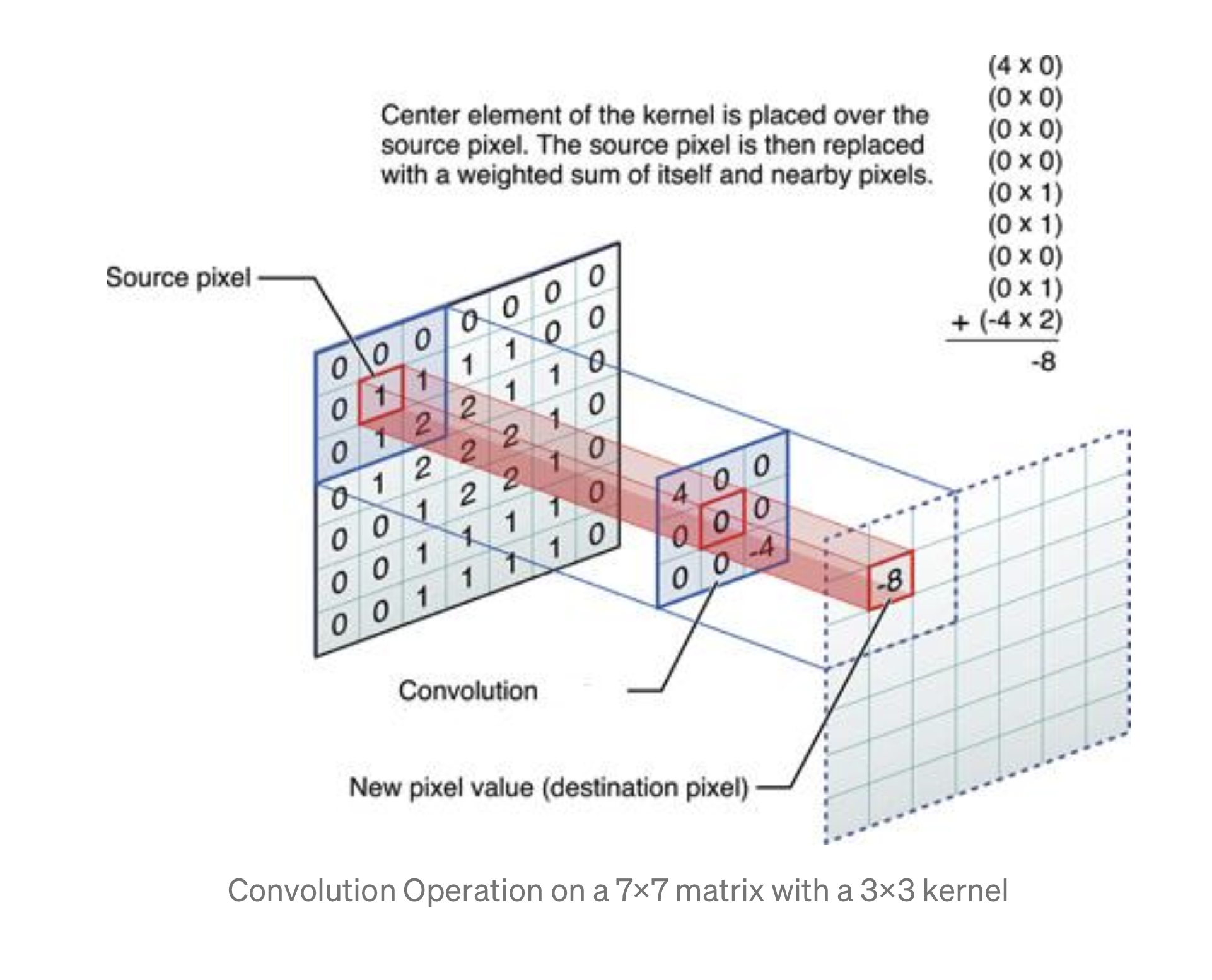
- In this exercise you manually applied a 3x3 array as a filter to an image of two people ascending an outdoor staircase. Modify the existing filter and if needed the associated weight in order to apply your new filters to the image 3 times. Plot each result, upload them to your response, and describe how each filter transformed the existing image as it convolved through the original array and reduced the object size. What are you functionally accomplishing as you apply the filter to your original array? Why is the application of a convolving filter to an image useful for computer vision? Stretch goal: instead of using the misc.ascent() image from scipy, can you apply three filters and weights to your own selected image? Describe your results.
- Another useful method is pooling. Apply a 2x2 filter to one of your convolved images, and plot the result. In effect what have you accomplished by applying this filter? Does there seem to be a logic (i.e. maximizing, averaging or minimizing values?) associated with the pooling filter provided in the example exercise (convolutions & pooling)? Did the resulting image increase in size or decrease? Why would this method be useful? Stretch goal: again, instead of using misc.ascent(), apply the pooling filter to one of your transformed images.
Finally, review the following images from class and then convolve the 3x3 filter over the 9x9 matrix and provide the resulting matrix. link to matrices
Thursday
For today's class you loaded and preprocessed the tf.dataset the tf_flowers, and then trained a CNN in order to predict whether a particular image was of one of five different types of flowers. For the first part of this exercise, instead of using the tf.keras.utils.get_file() to load your data, use tfds.load() to load a tensorflow dataset as illustrated in the section Using TensorFlow Datasets. Using the relevant parts from the entirety of the example script as a guide, fit a CNN model to your training data and validate using the beans dataset from Tensorflow datasets and then again train and validate using the eurosat dataset. Present your results and discuss the accuracy of each of model.
Additionally, go to the image augmentation exercise and read through and become familiar with the many individual examples presented. Towards the end of this exercise is the Apply augmentation to a dataset example, that illustrates a resize and rescale image augmentation implementation to the tf_flowers dataset. Apply this same method to both the beans and eurosat datasets. Did your model performance improve? How many epochs were you able to run and how much time did it take? Present your results and discuss the accuracy of your augmented output for tomorrow's class.
Module 3
Monday
Start with the Load CSV data script that we prepared during today's class. Following the Mixed data types section from the exercise, replace the titanic dataset first with the Metro Interstate Traffic Volume Data Set and then with the Iris Dataset. You can use the read_csv() command from the pandas package to pull these datasets from the following web addresses.
- https://archive.ics.uci.edu/ml/machine-learning-databases/00492/Metro_Interstate_Traffic_Volume.csv.gz
- https://storage.googleapis.com/download.tensorflow.org/data/iris_training.csv
Use the plot_model() command from tf.keras.utils to produce the plot that describes the input preprocessing step. Describe the plot of each model for the two dataset preprocessing steps. What does each box in the illustration represent? Are there different paths towards the final concatenation step? What is occurring at each step and why is it necessary to execute before fitting your model. Train each model and produce the output (not necessary to validate or test). Describe the model output from both the metro traffic interstate dataset and the iris flowers dataset. What is the target for each dataset? How would you assess the accuracy of each model? Are you using a different metric for each one? Why is this so? What is each one measuring?
For tomorrow, read and produce the script on Custom training: walkthrough in preparation for class.
Tuesday
Using the Custom training: walkthrough script we developed during today's class, write a 1-1/2 to 2-page report that provides a description of the following.
- the data used in the model
- how you created the
tf.dataset - how you specified your model architecture, including the input shape, the layers and other functions
- how you trained the model
- how you optimized the model
- how you estimated loss including a plot that describes that change per epoch
- how you evaluated the model with your test dataset
- how you made some predictions, including three new ones of your own and their results
For tomorrow, read and produce the script on Classify structured data with feature columns in preparation for class.
Wednesday
Using the Classify structured data with feature columns you prepared for today's class as a model example, train, validate and test a model that has wealth class as the target as follows.
- import the dataset city_persons.csv to your PyCharm environment
- Initially set the target to the least wealthy class, 2 in this case, and set all other wealth class outcomes to 0 (3,4 & 5)
- Train, validate and test your model
- Interpret and analyze your results. Did the model performance exhibit a particular trend?
For tomorrow, read and produce the script on Classify structured data using Keras Preprocessing Layers in preparation for class.
Thursday
Using the Classify structured data using Keras Preprocessing Layers you prepared for today's class as a model example, train, validate and test a model that has wealth class as the target as follows.
- Import the dataset country_persons.csv to your PyCharm environment
- Initially set the target to the least wealthy class, 1 in this case, and set all other wealth class outcomes to 0 (2,3,4 & 5)
- Train, validate and test your model
- Interpret and analyze your results. Did the model performance exhibit a particular trend?
Project 3
-
Using either the Classify structured data with feature columns script or the Classify structured data using Keras Preprocessing Layers with the
country_persons.csvdataset, specify, train and evaluate models that predict class of wealth versus all other classes as a binary target. Amongst the five possible binary targets (1 versus all others, 2 versus all other etc...), produce your results from the two models with the best and worst accuracy. -
Using the data and two models you produced in step 1, create a confusion matrix. You are welcome to use the following script. With your confusion matrix as a reference, analyze and discuss the two sets of results you produced.
-
Again using either the Classify structured data with feature columns script or the Classify structured data using Keras Preprocessing Layers with the
country_persons.csvdataset, specify, train and evaluate a model that predicts all class of wealth outcomes as a categorical target. Again create a confusion matrix in order to analyze and discuss your results. Revisit the Classify structured data with feature columns script or the Classify structured data using Keras Preprocessing Layers in order to modify your feature columns, in attempt to improve the accuracy of your model that uses all five categorical wealth classes as the target. Analyze and discuss your progress and results.
Step 1. Define your confusion matrix plot command
def plot_confusion_matrix(cm, classes,
                          normalize=False,
                          title='Confusion matrix',
                          cmap=plt.cm.Blues):
  """
  This function prints and plots the confusion matrix.
  Normalization can be applied by setting `normalize=True`.
  """
  import itertools
  if normalize:
    cm = cm.astype('float') / cm.sum(axis=1)[:, np.newaxis]
    print("Normalized confusion matrix")
  else:
    print('Confusion matrix, without normalization')

  print(cm)

  plt.imshow(cm, interpolation='nearest', cmap=cmap)
  plt.title(title)
  plt.colorbar()
  tick_marks = np.arange(len(classes))
  plt.xticks(tick_marks, classes, rotation=45)
  plt.yticks(tick_marks, classes)

  fmt = '.2f' if normalize else 'd'
  thresh = cm.max() / 2.
  for i, j in itertools.product(range(cm.shape[0]), range(cm.shape[1])):
    plt.text(j, i, format(cm[i, j], fmt),
             horizontalalignment="center",
             color="white" if cm[i, j] > thresh else "black")

  plt.ylabel('True label')
  plt.xlabel('Predicted label')
  plt.tight_layout()
Step 2. Create objects that describe the true and predicted target values
y_true = assign the true target values to this object
y_pred = assign the predicted target values to this object
Step 3. Plot your confusion matrix
cnf_matrix = confusion_matrix(y_true, y_pred,labels=[add labels here])
np.set_printoptions(precision=2)

plt.figure()
plot_confusion_matrix(cnf_matrix, classes=[add labels here],
title='title your plot')
plt.show()
Module 4
Wednesday
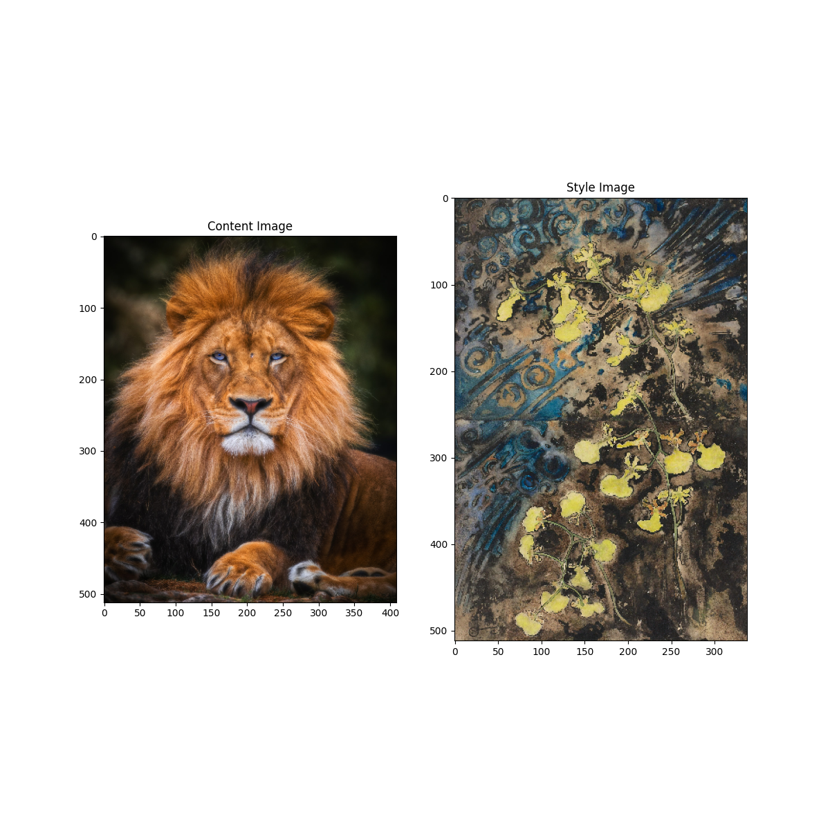
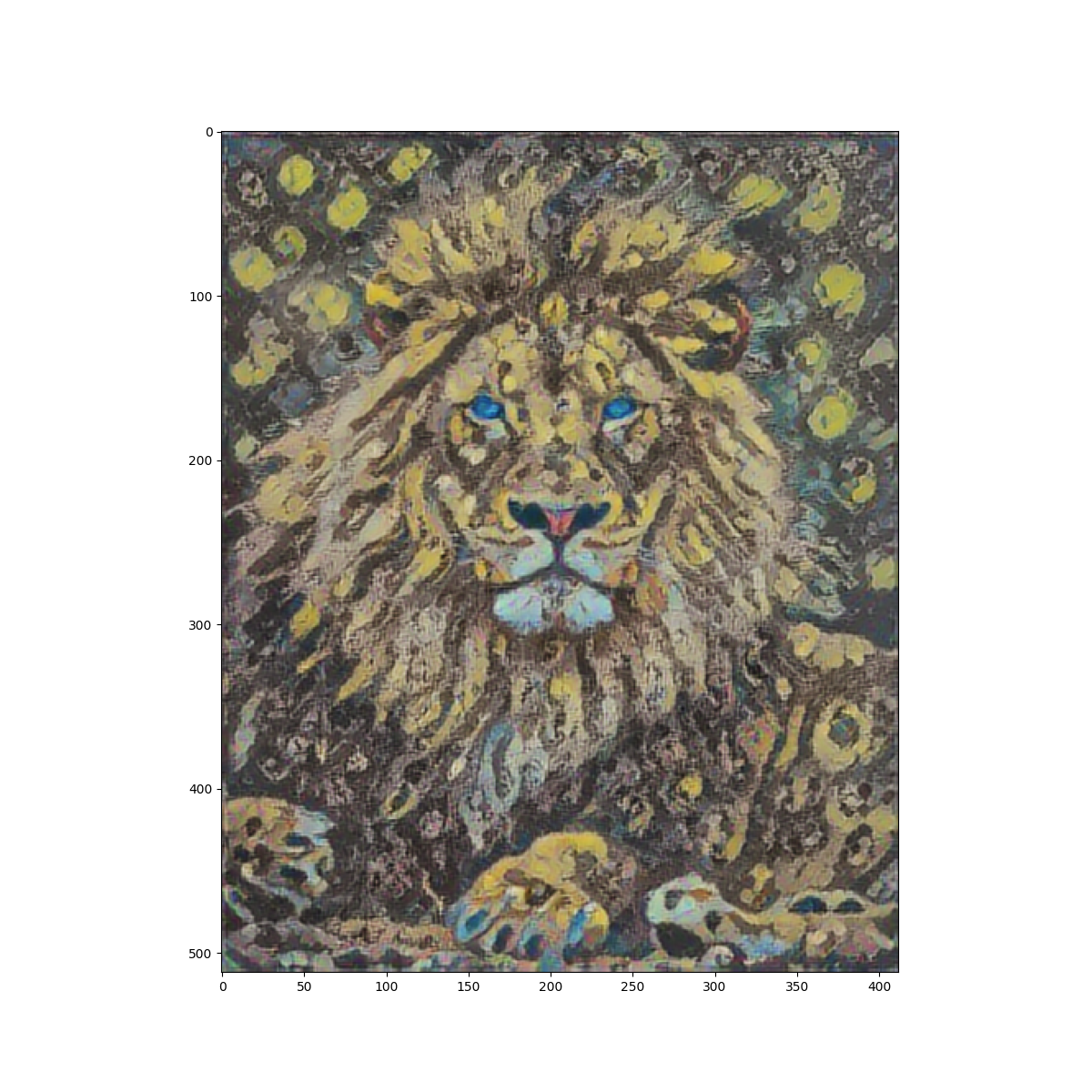
Using the Neural Style Transfer script we developed during today's class replace the content and style images with two images of your own selection. Synthesize the two images by applying the following elements from the exercise.
- Define content and style representations
- Extracting style and content
- Implementing the style transfer algorithm
- Apply regularization term on the high frequency components
Describe your implementation of neural style transfer to your content and style images. How did the application of the four steps from above produce your resulting work of art. Comment on what your work means in terms of your development as a data scientist at William & Mary with forethought to the future (please feel free to take as much artistic license as you wish when answering this last question).
Stretch goal: Using the the Deep Dream script, produce another version of your artwork.
For tomorrow, we will work on producing the script from the tensorflow exercise Text generation with an RNN during class in continued preparation for Project 4.


Thursday
Using the Text generation with an RNN script we developed during today's class, use the shakespeare.txt file to generate your own text that imitates the script from Shakespeare. Produce your generated text and describe how it was produced, addressing the following aspects.
- Processing, vectorizing and predicting text
- Building and training the model
- Generating text
Stretch goal: Add the Advanced:Customized Training procedure at the end of the exercise by specifying a starting point and implementing curriculum learning.
Project 4
Using the Text generation with an RNN from Thursday, replace the shakespeare.txt with a screen play script from your favorite movie. Use the RNN model to generate new text from the source document and then use that machine generated output as the basis for a 5 to 8 minute production on Monday. Be sure to assign a role for each team member such that everyone has a chance to perform. Use the text generated from your RNN model as the basis for your theatrical production, but also feel free to modify it as you please in order to make your presentation more entering. By Monday evening, answer the following questions as a group and post to your GitHub index.
- How did you modify the data and python script in order to generate comprehensible text?
- Did your output seem to generate text that was relying more on the entire corpus of your screen play (i.e. more associated with long term memory) or was it also able to incorporate some more immediate sequential associations (i.e. more associated with short term memory)?
- Did you make any changes to the model itself?
- Were there any unexpected or surprising phrases or statements that were generated by your RNN?
As a stretch goal, for your Monday morning presentation, produce one or two images (using the neural style transfer and/or deep dream methods) that you can use as a virtual background to supplement your RNN generated and inspired theatrical production.
Present your Results
Summary
For the final assignment of this course, record an eight to twelve minute presentation of the applied machine learning model you will use as a prototype for your proposed future research plan. Your recorded presentation will be due by 5PM on August 8th.
Step 1. Write an abstract and give your presentation a title
Draft an abstract and give your presentation a title. Review and edit your abstract, which should be less than a page in length, single spaced. Post your abstract to your index in advance of the deadline.
Step 2. Prepare the slides for your presentation
Prepare to speak eight to twelve minutes and include at least one presentation slide that addresses each of the following elements from your work.
-
A problem statement that introduces your selected topic, identifies significant goals associated with the implementation of your applied machine learning method, demonstrates why your problem is important, and describes and analyzes the complex nature of your problem including any process oriented causes and effects. Conclude your problem statement with a stated central research question. You are welcome to articulate a central research question in broad and general terms, given the abbreviated time frame for this investigation.
-
A description of the data that you are using as input for your applied machine learning methodology, including the source of the data, the different features (variables) and well as their data class (i.e. continuous or discrete). Be sure to include a description of your dataset size (number of rows / observations as well as number of columns / variables / features) and provide context on how the data was collected as well as the source.
-
Provide the specification for your applied machine learning model that presented the most promise in providing a solution to your problem. Include the section from your script that specifies your model architecture. Provide a brief description of how you implemented your code in practice.
-
Conclude with a section that preliminarily assesses model performance. If you have results from your implementation, you are welcome to add those in this section. Compare your preliminary results with those from the literature on your topic for a comparative assessment. If you are not able to produce preliminary results, provide a cursory literature review that includes 2 sources that present and describes their validation. With more time and project support, estimate what an ideal outcome looks like in terms of model validation.
Step 3. Record your presentation
Record your eight to twelve minute long presentation and provide a link to it via your zoom or panopto folder on your GitHub index. Using any combined screen and audio recording device is perfectly acceptable (Mac, Windows, Linux). Send your link to me as a message in slack in advance of the August 8th deadline.
Links to Responses
- Huatao Chen
- Michael Cusack-Nelkin
- Lydia Danas
- Liz Goodwin
- Dylan Hartman
- Cori Ingram
- Maggie Kettelberger
- Alexandra MacNamara
- Aashni Manroa
- Thomas Miller
- Alaa Mokbel
- Ethan Nelson
- David Olsen
- Annabel Richter
- Gwen Wagner
- John Willis
- Tyler Yeatts
- Julia Lewis
Links to Responses
- Amy Hilla
- Emma Schmidt
- Natalie Larsen
- Alleah Thornhill
- Sarah Grace Lott
- Jacinta Das
- Margaret Delaney
- Austin Anderson
- Wayne Wu
- Andrew Evan
- Alejandro Eulacio
- Sean Frankel
- J.Mo Yang
- Jacob Atagi
- Antonio Marra
- Richard Bartlett
- Victoria Chang
- Conrad Ning
- Dominic Skeete
- Frank Qiu
- Pablo Solano
- Tommy Williams
- Suditi Shyamsunder
- Rachel Li
- Jeremy Swack
Links to Responses
- Alex Raposo
- Luke Denoncourt
- Caroline Wall
- Daniel Highland
- Maddy Mulder
- Roger Clanton
- Matthew Cheng
- Caroline Freshcorn
- Caitlin Bryant
- Maddie Sharpe
- Alex Huang
- John Hennin
- Devika Puri
- Annette Lopez Davila
- Kathryn Johnson
- Jennifer Lam
- Anthony J. Ventura
- Paul Brenkus
- Sarena Oberoi
- Lily Bartholomaus
- Darrin Lilly
- David Huang
- Tommy Williams
- Youjin Lee
- Chai Hibbert
