Adding transportation facilities & health care services
To start the final part of project 3, head back to the HDX website that we used all the way back during the first few weeks of the semester and enter the name of your selected LMIC. Again, I will select Liberia and begin to browse through the available data. Identify the road network dataset for your LMIC and then select it. Select the download button on the subsequent webpage and obtain the available data. Move the folder you just downloaded (including the shapefile and all of its other associated files) to your working directory.
Import the roads shapefile into RStudio using the read_sf() command.
LMIC_roads <- add_command_here("data_folder/LMIC_roads.shp")
Using the polygon you created at the end of the previous exercise use the st_crop() command to crop your LMIC_roads object to just those roadways that are located within the adm2 or adm3 previously selected.
adm2_roads <- add_command_here(LMIC_roads, unioned_adm2_borders)
Use the table() command to review the different classifications of roads that populate your adm2. Most likely the variable you will be interested in producing a table that describes the different discrete values is named CATEGORY.
add_command_here(object$variable)
Take each of these different discrete outcomes within your roads sf object and use the filter() command to subset based on each different classification.
primary <- adm2_roads %>%
  add_command_here(VARIABLE == "Primary Routes")

secondary <- adm2_roads %>%
  add_command_here(VARIABLE == "Paved")

tertiary <- adm2_roads %>%
  add_command_here(VARIABLE == "Tracks")
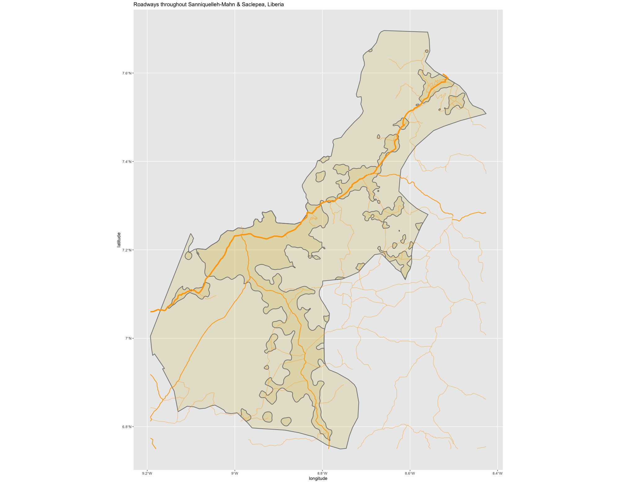
Use ggplot() to produce a plot that describes the location of all urban areas as well as the transportation network throughout your selected adm2.
ggplot() +
  geom_sf(data = combined_adm2s_border,
          size = 0.75,
          color = "gray50",
          fill = "gold3",
          alpha = 0.15) +
  geom_sf(data = combined_urban_areas,
          size = 0.75,
          color = "gray50",
          fill = "gold3",
          alpha = 0.15) +
  geom_sf(data = primary_roads,
          size = set_size,
          color = "color") +
  geom_sf(data = seondary_roads,
          size = set_size,
          color = "color") +
  geom_sf(data = tertiary_roads,
          size = set_size,
          color = "color") +
  xlab("longitude") + ylab("latitude") +
  ggtitle("Roadways throughout your selected adminitrative units")
The previous code will produce the following plot for the two Liberian administrative subdivisions that were previously selected and unioned into a single sf object.
Go back to the HDX website for your LMIC and download the data that describes health care facilities. Use the read_sf() command to load the data into RStudio. Use st_crop() to crop the health care facilities to your selected adm2 or adm3 area. Use table() to identify all of the different types of health care facilities. Subset each of the health care facility types in the same manner you previously subset transportation facility classifications.
hospitals <- adm_hcf %>%
  add_command_here(add_variable_here == "hospital")

clinics <- adm_hcf %>%
  add_command_here(add_variable_here == "clinic")

other_hcfs <- adm_hcf %>%
  add_command_here(add_variable_here == "doctors" | add_variable_here == "dentist" | add_variable_here == "pharmacy")
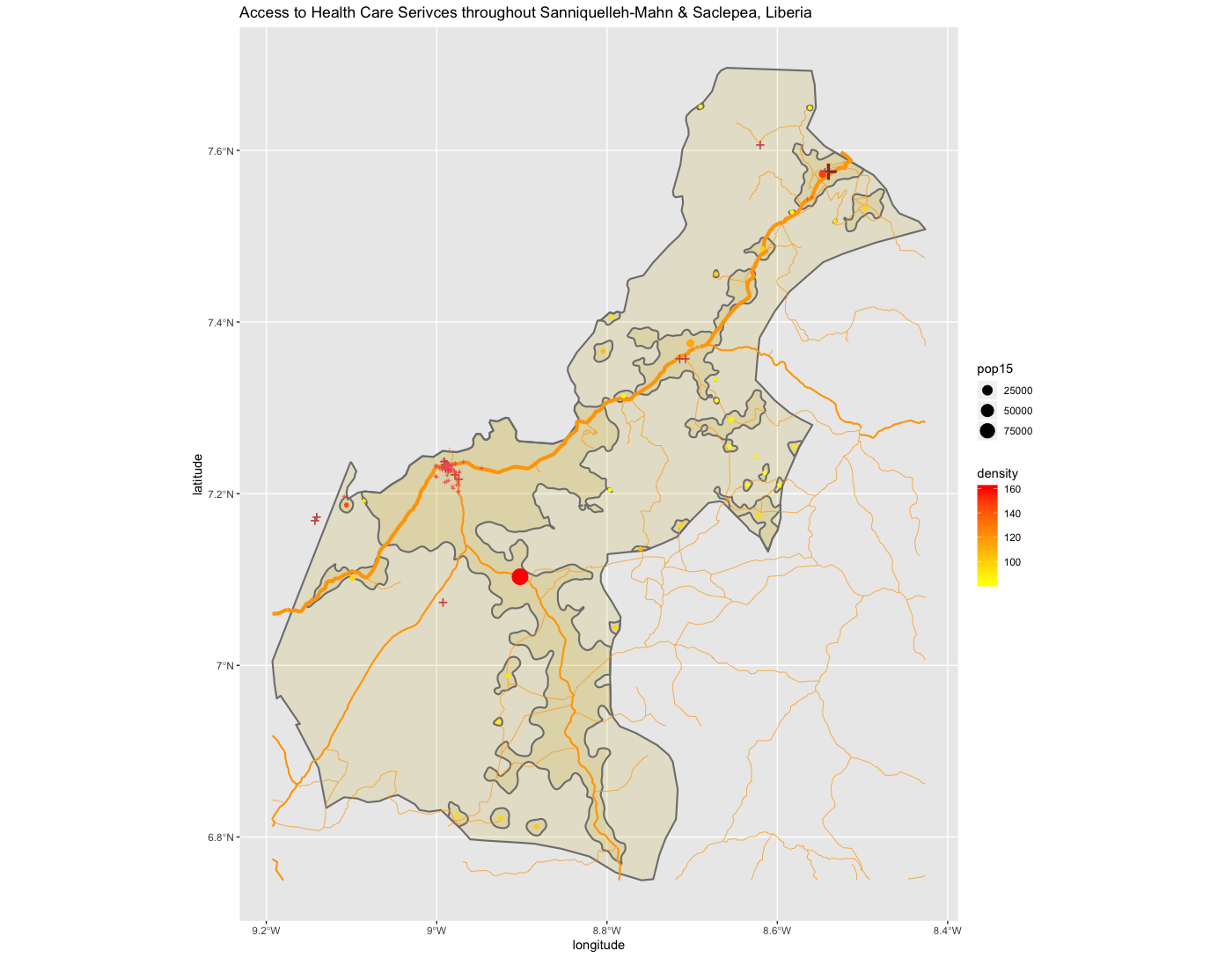
Add each health care facility type to your plot.
ggplot() +

...

  geom_sf(data = hospital,
          size = add_size,
          color = "color") +
  geom_sf(data = clinic,
          size = add_size,
          color = "color") +
  geom_sf(data = ohcf,
          size = add_size,
          color = "color") +

  ...

  ggtitle("Access to Health Care Serivces throughout Sanniquelleh-Mahn & Saclepea, Liberia")
The previous plot will produce the following output.

Finally, add the scale that describes the size and density of each urban area. Produce the plot that describes access to health care services via transportation facilities throughout your selected and combined adm2 areas.
Project 3. Individual Deliverable
Upload the spatial plot that describes the de facto location of human settlements and urban areas, the center lines of classified roadways and the location of health care facilities by type throughout your selected and combined adm2, adm3 or adm4 areas.
Accompany your plot with a written statement that provides answers to the following information.
- Total population of selected and combined adm2, adm3 or adm4 areas and the total number of distinctly defined human settlements or urban areas
- A description of the distribution of sizes and densities of all human settlements and urban areas throughout your selected and combined adm2, adm3 or adm4 areas
- A description of the roadways and your estimate of the transportation networks level of service in comparison to the spatial distriubtion of human settlements and urban areas
- A description of health care facilities and your estimate of service accessibility in comparison to the spatial distriubtion of human settlements and urban areas
Each team member should be prepared to present their final draft results on Friday, November 15th during the informal group presentations. Upload your finished product to the slack channel #data100_project3 no later than 11:59PM on Sunday, November 17th.